Turfgrass Growth Potential (GP)
Find the temperature-based growth potential of cool- and warm-season turfgrass
Growth potential equation
| Format | Cool-season grass (C3) | Warm-season grass (C4) |
|---|---|---|
| Equation | Cool-season grass (C3) GP = e−½((T − 68)/10)² GP = e−½((T − 20)/(50/9))² | Warm-season grass (C4) GP = e−½((min(T, 88) − 88)/12)² GP = e−½((min(T, 31) − 31)/7)² |
| Excel | Cool-season grass (C3) | Warm-season grass (C4) |
| R | Cool-season grass (C3) | Warm-season grass (C4) |
| Python | Cool-season grass (C3) | Warm-season grass (C4) |
GP ranges from 0 to 1 (or 0 to 100%). T (shown as temp_ftemp_c in the formulas) is average
air temperature in °F°C. Warm-season GP stays at 1 above 88°F31°C.
How to use growth potential
- Choose the grass and temperature. Decide whether you are calculating GP for cool-season (C3) or warm-season (C4) grass. Find the average air temperature for the day or month you want to assess.
- Use the matching constants. With Fahrenheit temperatures, the optimum and scaling constant are 68°F and 10 for C3, or 88°F and 12 for C4. With Celsius temperatures, use 20°C and 50/9 for C3, or 31°C and 7 for C4.
- Calculate GP. Subtract the optimum temperature from the average temperature, divide by the scaling constant, square that result, multiply by −0.5, and raise e to that power. For C4 grass, use the optimum temperature when average temperature is above the optimum temperature; GP remains at 1 when C4 grass is grown in high temperatures.
- Read the result. GP runs from 0 to 1 (or express on a scale of 0 to 100%). A value of 0.5 represents half of the maximum temperature-based growth potential; a value near 1 indicates temperatures near the model's optimum.
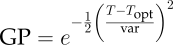
where,
- GP
- Growth potential, on a scale from 0 to 1.
- e
- The mathematical constant, approximately 2.71828.
- T
- Average air temperature, in °F or °C. Use the matching unit for T, Topt, and var.
- Topt
- Optimum temperature: 68°F for C3 or 88°F for C4; 20°C for C3 or 31°C for C4.
- var
- Temperature scaling constant, which controls how quickly GP falls as temperature moves away from the optimum: 10 for C3 or 12 for C4 with °F; 50/9 for C3 or 7 for C4 with °C.
C4 growth does not have the same photorespiration-driven decline above its optimum as C3 growth, so C4 GP remains at 1 above the optimum temperature. Temperature-based GP is a planning estimate: actual growth also depends on factors such as water, nitrogen, light, and the grass variety.
About growth potential
We developed the growth potential model to explain the many ways that temperature impacts turf growth. The model considers turf growth to be good when the growth potential (GP) is between 50% and 100% (the best possible growth occurs at a GP of 100%). However, when weather conditions are either too hot or too cold for optimal turf growth, the GP falls below 50%, and turf becomes progressively more stressed. When the GP falls to 10% or lower, growth is extremely limited.
Growth potential gallery
Growth potential calculator
Growth potential
Monthly values
| Jan | Feb | Mar | Apr | May | Jun | Jul | Aug | Sep | Oct | Nov | Dec | |
|---|---|---|---|---|---|---|---|---|---|---|---|---|
| Avg. temp °C | ||||||||||||
| Cool GP % | ||||||||||||
| Warm GP % |
Temperature averages from 2021 to 2025 (ERA5-Land)
Documents
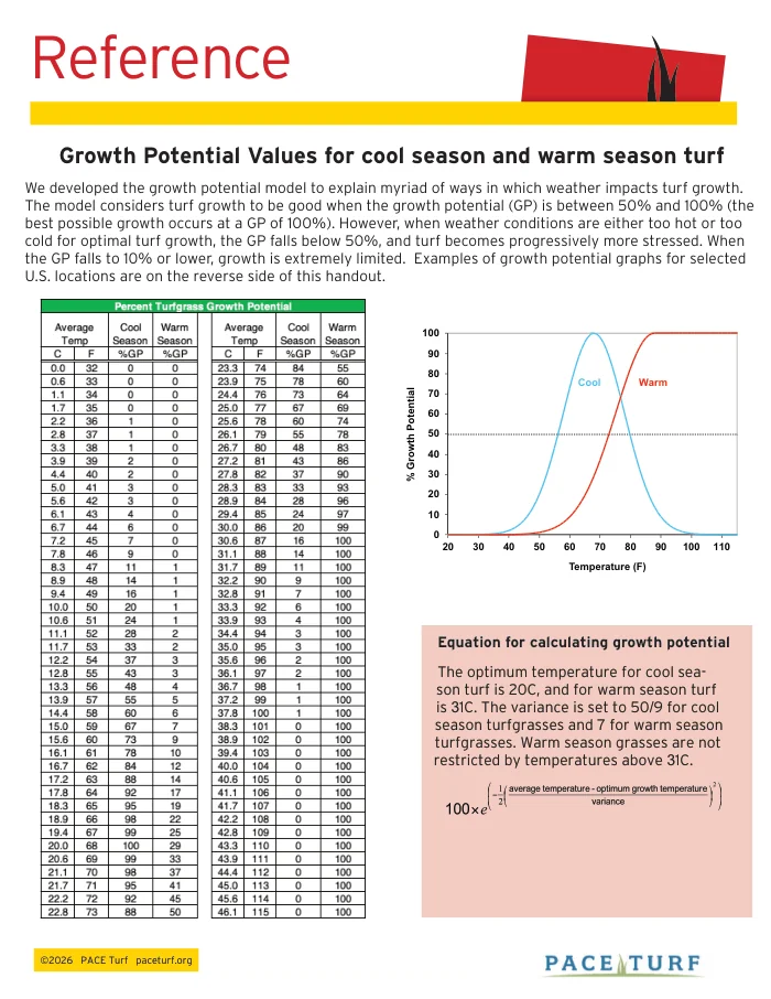 Growth Potential Values for cool-season and warm-season turf
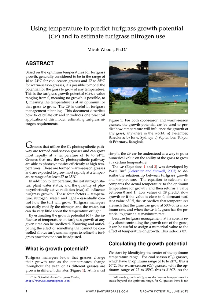 Using temperature to predict turfgrass growth potential (GP) and to estimate turfgrass nitrogen use
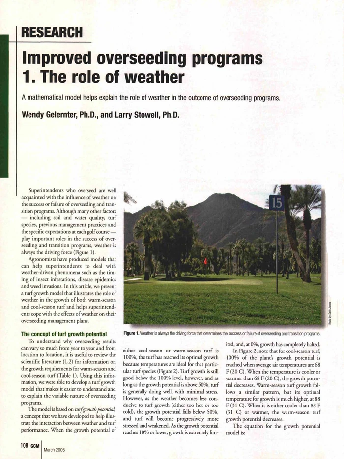 Improved overseeding programs: The role of weather
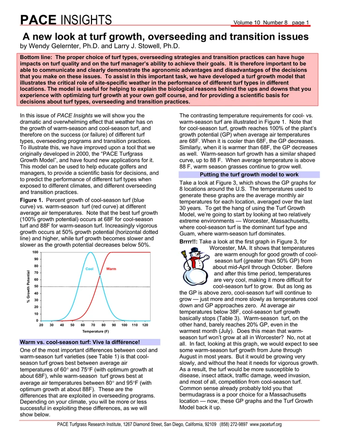 A new look at turf growth, overseeding and transition issues
Case studies
Sudbrook Moor Golf Club Grantham, United Kingdom
James Sergeant used GP to set clipping volume targets, then measured clippings to guide nitrogen applications. Annual nitrogen use fell from about 15 g/m² under the previous years' program to nearly 5 g/m². The bent-Poa greens continued to perform well.
PACE Turf report James Sergeant on XPender Harbour Golf Club British Columbia, Canada
After catastrophic winter kill in 2017, Jason Haines used GP to show members why greens recovery was slow: spring temperatures were poor for growth compared with previous years. During the summer, growth potential showed short dips, telling him when to ease off stressful maintenance and giving him the data to explain why. Jason suggests posting GP alongside green speed to explain conditions.
Jason Haines blogAlabama golf course Alabama, United States
An Alabama golf course used GP to help decide which month to aerify creeping bentgrass greens and optimize recovery time. The golf course also looked at GP ahead of an April tournament, because they considered fertilizing a bermudagrass rough to make it more challenging. GP graphs showed growth would be below 20% at that time of year and that made enough new rough growth unlikely.
USGA Green Section RecordComparing season length
Summing daily GP over a year gives a proxy for growing-season length, which makes it easy to compare locations on temperature. For example, one year works out to about 138 days for Minneapolis and 165 for New York City. You can scale inputs by that ratio: 8 mm of sand topdressing in New York would be about 6.7 mm in Minneapolis. The same approach works for nitrogen rates and mowing frequency.
Asian Turfgrass Center articleFAQs
How does growth potential relate to nitrogen use?
GP shows how favorable the temperature is for growth. We use GP value with a standard daily nitrogen amount to estimate nitrogen demand at your location. This gives you a starting point for planning. Compare the estimate with actual growth before adjusting nitrogen applications. See Standard nitrogen for how our weather report uses GP.
How does growth potential relate to clipping volume?
GP estimates growth conditions from temperature, and clipping volume measures how much grass you actually harvested. High GP does not guarantee high clipping volume because nitrogen supply, water, growth regulators, and other conditions also affect growth. Comparing measured clippings with the amount expected from recent GP can help you decide whether to adjust nitrogen. We call this comparison Turf GvX.
Is there a separate growth potential model for kikuyugrass?
Yes. Kikuyugrass GP peaks at an average air temperature of 24°C. Its equation is:
GP = e−½((T − 24)/var)²
Here T is average air temperature in °C. Use var = 6.1 when T is 24°C or lower, and var = 3.9 when it is above 24°C.
gpk <- function(temp_c) {
  var <- ifelse(temp_c <= 24, 6.1, 3.9)
  exp(-0.5 * ((temp_c - 24) / var)^2)
}